Using Scatter Plot To Visualize Solution Space In MATLAB

May 23, 2018
matlab optimization
2 min read

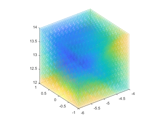
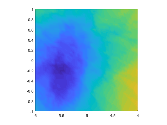
I have a cost function of 3 parameters, whose solution space is discontinuous and should have local minimums. In order to observe the space to get a grasp of how swampy the space is, I plot a scatter plot of many points in the solution space, and each point’s color indicates its value. Following this video, I also plot a slice to visualize the values in that slice. Here are the code and the plots.

% create scattered plot to visualize the solution space
% create the meshgrid
x = [-6:0.05:-4];
y = [-1:0.05:1];
z = [12:0.05:14];
[X,Y,Z] = meshgrid(x, y, z);

% C stands for color, and stores the value of the cost function at each point
C = X;
for i = 1:size(x,2)
    for j = 1:size(y,2)
        for k = 1:size(z,2)
            C(i, j, k) = costFunction([x(i), y(j), z(k)], extraParameters);
        end
    end
end

% plot scatter plot
figure();
scatter3(X(:),Y(:),Z(:), 3, C(:), 'filled') % each point is of size 3 and is filled
axis equal;

% plot a slice of of the solution space
figure();
h = slice(X,Y,Z,C,[],[],13.3);
h.FaceColor = 'interp';
h.EdgeColor = 'none';
axis equal;

The scatter plot:

The slice plot:

The darker blue area is where the minimum lies. This helps us visualize that the solution space is generally continuous, with some local minimums here and there.

Boyi's Log

Using Scatter Plot To Visualize Solution Space In MATLAB